The third contingency - illustrated in Fig. 6c - consists
of the loss of a generator ( 700MVA) in Plant 1 shown in Fig.
5, which is located in the ``center'' of the
load region. We observe from the scatter plot that this contingency is
much severer than the two preceding ones (
700MVA) in Plant 1 shown in Fig.
5, which is located in the ``center'' of the
load region. We observe from the scatter plot that this contingency is
much severer than the two preceding ones (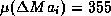 MW)
and rather variable (
MW)
and rather variable (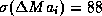 MW). Moreover, in
contrast to the line tripping contingency it is difficult to suggest a
priori a small number of parameters liable to ``explain'' this
contingency.
MW). Moreover, in
contrast to the line tripping contingency it is difficult to suggest a
priori a small number of parameters liable to ``explain'' this
contingency.
Thus we will illustrate the overall systematic approach suggested in
§2, combining regression trees and multilayer perceptrons. To
validate the model  , we keep aside 796 test
states among the 4041 relevant states of this contingency, and we use
the remaining 3245 states as learning set. So as to avoid missing
some important information, a rather large list of 138 pre-disturbance
candidate attributes is used.
, we keep aside 796 test
states among the 4041 relevant states of this contingency, and we use
the remaining 3245 states as learning set. So as to avoid missing
some important information, a rather large list of 138 pre-disturbance
candidate attributes is used.
The first step consists of building a regression tree. This selects among the 138 candidate attributes those which are most strongly correlated with the severity. In the present case, 15 test attributes are selected, comprising by decreasing order of importance the reactive flow through the 400/225kV transformers in substation 2, the total reactive EHV compensation of the region, the active flow through 400/225kV transformers in Plant 1 substation and the reactive reserve available in this plant. The regression tree remains however quite simple, since it is composed of 18 test nodes and 19 terminal nodes.
The model is further refined by exploiting the continuous modelling
capabilities of multilayer perceptrons. To this end, we use a
multilayer perceptron with 15 input neurons, corresponding to the 15
attributes selected by the tree, 20 (this number is arbitrarily fixed)
hidden neurons, and a single output neuron corresponding to the
severity appropriately normalized in the interval  .
The BFGS procedure, applied to adjust the 340 weights of the latter
model so as to reduce the overall MSE in the learning set, converged
after 305 passes through the learning set. Using the multilayer
perceptron to approximate the value of the severity of the test states
yields a mean error of -0.8MW and standard error deviation of
43MW. Figure 7b shows the scatter plot of the
pre-computed post-contingency margin vs. the estimated one using
eqn. (1).
.
The BFGS procedure, applied to adjust the 340 weights of the latter
model so as to reduce the overall MSE in the learning set, converged
after 305 passes through the learning set. Using the multilayer
perceptron to approximate the value of the severity of the test states
yields a mean error of -0.8MW and standard error deviation of
43MW. Figure 7b shows the scatter plot of the
pre-computed post-contingency margin vs. the estimated one using
eqn. (1).
Further, the use of this margin to classify test states with respect to to a threshold of 255MW (see Fig. 7b) yields an error rate of 4.9%. Given the lower bound of the margin computation accuracy (and the thereby induced error rates shown in Table 1), we conclude that the proposed approach yields a very satisfactory level of accuracy, for all three contingencies.